Numpy efficiency and lumpy sigmoids

The problem

Some time ago I wrote about the relative efficiency of the Python numpy library when comared with Octave and C, and I thought it would be interesting to see how numpy compares with Python itself.

For those unfamiliar with numpy, it is a wonderful open-source extension to standard Python which allows  powerful multidimensional array handling.

One of numpy's most powerful features is "broadcasting". This allows a single operation to operate on entire arrays. This is important as the underlying code for manipulating arrays in numpy is actually written in highly optimised FORTRAN and C. As a result, although there is an overhead associated with creating the numpy array and any calls to the underlying code, the actual array manipulation is extremely efficient and fast.

Python is, of course, an interpreted (byte compiled) language, and so doesn't have the efficiency associated with compiled languages. Back in the days of yore, in order to perform an operation (say) multiplying two arrays of random numbers together, one might in the absolute worst case do something like:

   for m in range(n):  
     x.append(random.random())  
     y.append(random.random())  
   z = []    
   for a, b in zip(x, y):  
     z.append(a * b)  

As these sorts of operation are quite commonplace, since Python 2.0 list comprehensions have been introduced, which allow us to do the same code as above much more elegantly and efficiently.

   x = [random.random() for k in range(n)]  
   y = [random.random() for k in range(n)]  
   z = [a*b for a, b in zip(x, y)]  

List comprehensions have the additional advantage that they are much faster (about 1.8x to 1.9x faster on my system running Python 3.4).

So I decided to compare the performance of the list comprehension above with that of numpy broadcasting, where the list comprehensions above would be replaced with the wonderfully clear and understandable

   x = numpy.random.rand(n)  
   y = numpy.random.rand(n)  
   z = x*y  

We would expect the relative performance of numpy versus list comprehension to be dependent on the size of the arrays involved. With very small arrays, the overhead of creating the numpy array and handling the calls to the underlying code wouldn't be worth it and numpy might even in a worse case be slightly less efficient. But as the array length, n, increases we would expect the performance to increase and plateau out to a maximum, with the performance curve being a classic sigmoid shape.

So I performed some tests determine the average time to multiply arrays of random floats together using list comprehensions and numpy broadcasting, for arrays of a number of lengths from 1 to 5,000,000. Timing is to the nearest microsecond, using the Python datetime library.

The results

The results, as expected, give a classic sigmoid shape. For larger array sizes we see a performance ratio of about 12:1.

I'd originally intended to write this post purely about the relative efficiency of numpy and list comprehensions. But I got quite a surprise when I looked at the graphs of the performance tests.

So as you can see, we get a broadly sigmoid curve, with there being little or no advantage for arrays shorter than about 10³ elements. (Note the logarithmic scale). Now although we would expect quantisation noise, caused by the fact that we are only timing accurate to the microsecond, and really short arrays will be processed faster than that for lower values of n. But the figures were averaged over 1,000 runs which should smooth things out somewhat.

But it's very noisy. Also the curve for Windows is much noisier than that for Linux. There are two possible causes of this.

Garbage collection. This is when Python periodically pausea to release objects from memory which are no longer required. This can be turned off by importing the Python gc library and enabling and disabling garbage collection at the appropriate times using gc.enable() and gc.disable(). Note that both systems have an abundance - 16 GB - of memory.

This is far an away the most likely cause. But it could also be...

Multiple cores. Python programs are sometimes moved between CPU cores during operation by the Global Interpreter Lock and also the operating system itself, for whatever reason, might also decide to unload something from one core and move it to another or operate an application across multiple cores. This can obviously make attempting to time stuff accurate to the microsecond difficult. It's possible to control this using the task manager in Windows and by using the taskset -c command in Linux.

So what effect does this have. First let's try disabling garbage collection.


Clearly there's a dramatic improvement in the Windows curve but the Linux one is fundamentally much the same. So what effect would binding the Python interpreter to a single CPU core have? To be honest, very little.

 

Curiously, on all the runs, there is an inflexion in the Linux curve at about n = 10⁵ which can't be explained by garbage collection etc. This consistently occurs in the same place every time the software is run, so something must be causing it but I have no idea what. (I've ruled out obvious things like paging/swapping, due to the huge amount of physical memory).

Conclusions

1. We do, as expected get a sigmoid curve.
2. Numpy begins to get more efficient in this simple case at n > 10³, but if we were performing significantly more complex calculations than generating and multiplying random numbers numpy would begin to win for lower n. (Perhaps this is something to be tested another time). 
3. For large n (> 10⁵), numpy outperforms a Python list comprehension typically by a factor of 12.
4. Quantisation noise occurs at lower values of n but can be smoothed out by averaging over several runs. Noise is significantly worse, as is overall noise/discontinuity in the results under Windows. This is unlikely to be related to external system load, as both systems are relatively lightly loaded, and is more likely to be due to Linux coping better under load conditions. (It is noticeable, for example, that even at 100% load, most Linux systems will have a decent interactive response. In fact the Linux system on which these test were performed is significantly more heavily loaded than the Windows system, has a slower CPU and actually completed the tests approximately 30% faster than the Windows one.)
5. Clearly something must be causing the inflexion in the Linux curve at n ~ 10⁶. But I don't know what. 

Making a timelapse video with a webcam and Linux

Out of my window I can see a building site on the site of the old BBC studios on Oxford Road, Manchester. As there's going to be a few years building work, I thought it would be interesting to produce some sort of time-lapse film of the works from my office window.

This post explains how I did it.

I have an existing Ubuntu Linux system which runs 24x7 doing a variety of different things, and so I decided as this was likely to have a far better uptime than my Windows system to use this to do the hard work.

First connect your webcam

So the first thing I did was to install a (cheap) USB web-cam bought from my local PC dealer for about a tenner. Make sure that the webcam you get is either marked as Linux compatible or compliant with the UVC standard. Mine just worked straight out of the box.

The most difficult thing was physically fixing the webcam in place. Most of them come with a fairly flimsy plastic clip designed to secure it to the top of a monitor, but that was unsuitable for my purposes. As I want to leave it in fundamentally the same position for several months, I also needed to be confident that it was moved, say for cleaning, then I could reposition it reasonably accurately.

I ended up securing the webcam to the top of a old tin of Chinese tea with elastic bands and wedging the entire thing against the window fittings, so it shouldn't move overly much. Not particularly elegant. But it works beautifully.

Now select your software

I want the webcam to take a photo every minute or so and tried various bits of client software to do this. The one I selected as having the best combination of features for my requirements. Eventually I settled on the fswebcam client, which can be installed using the command

$ sudo apt-get install fswebcam

After a bit of experimentation I found the command that gave me the best results was

$ /usr/bin/fswebcam  --background --device /dev/video0 --loop 60 --resolution 1280x720 --skip 10 --frames 3 --delay 5 --bottom-banner /home/tim/archive/tim/pix/\%Y-\%m-\%d_\%H:\%M:\%S.jpeg

The options do the following things:

--background flag tells the device to run in the background
--device specifies which device to use for capture, in this case the (rather obvious) /dev/video0
--loop makes the camera fire every 60 seconds
--resolution sets the image resolution. 1280 x 720 results in JPEG image of anywhere between about 40 and 140 KB depending on how much the image can be compressed
--skip 10 --frames 3 --delay 5 makes the camera makes the camera delay for 5 seconds, then skip the first 10 frames, then take an average image over the next 3 frames. I did this because I found that the (cheap) camera I had used had difficulty coping with changing light levels, and so, for examples, photos taken in the morning as the sun rose were completely overexposed. I recommend playing around with these settings until you get something which suits your requirements.
--bottom-banner produces a timestamped banner at the bottom of the image.

This is the sort of image it produces.

So I now had something which was taking an image every minute and placing it in the /home/tim/archive/pix directory with a filename something like 2016-02-23_10:12:00.jpeg (this is important as we want to be able to stitch many images together sequentially).

Note, however, that a 140 KB file being generated every minute does tend to chew your disk up: it will generate about 200 MB of output a day or, if you prefer, about 70 GB a year. My /home/tim/archive directory is actually a mount-point for a 1 TB disk, and so there's plenty of room, but if you have limited space then either reduce the image resolution or the frequency with which images are captured. I also periodically manually thin out the images (using rm), discarding, for example, any which are taken between 18:00 and 08:00 the following day as there is no building work going on during these periods. This reduces the daily output from 200 MB to about 80 MB.

Note also that if the frequency with which you want to take photos is measured in minutes, then rather than using the --loop option you could just as easily do it with a cron job, by creating a crontab using the

$ crontab -e

command. This would have the advantage that you could have much finer-grained control over the times at which pictures were taken - e.g. Monday to Friday, 08:00 to 18:00.

Although my system typically has uptimes of several months, it is rebooted occasionally. So I wanted to make sure that the image capture started automatically when it did so. I therefore put the fswebcam command above in the /etc/rc.local configuration file.

One bit of strangeness is that fswebcam doesn't work if you aren't logged in, even if it run as a cron job or with something like nohup. This doesn't matter on my system as I am automatically logged in at boot, but be aware of it and, if you find a solution please let me know!

Now stitch your frames together

I think that, really, most people won't be interested in a time-lapse video longer than about one or two minutes duration. So assuming that we're showing maybe 24 frames per second (FPS), then that's about 1,440 frames per minute. Now, taking a picture every minute for eight hours a day, means that per day my setup produces about 480 frames per day, or, if you prefer 20 seconds of video if I were to show all the frames.

Assuming that the timelapse is to be over a longer period, then it's necessary either to take fewer frames in the first place, by controlling the frequency with which fswebcam acquires images as discussed above or, alternatively, only selecting certain images. I chose this latter option, as I have plenty of storage space I didn't know if, at some stage, I might want to do a more granular video.

Now, my preferred way of stitching these frames together is ffmpeg. This is no longer included in the standard Ubuntu distribution and, instead, there is a fork of it called avconv

This has a really cool feature which allows sequentially numbered frames to be stitched together in to a video. Now as I only want to select some frames, I wrote a very simple Python script which will select the frames I want between certain hours of the day, days of the week and also introduce a "gap", so only selecting one frame in (say) 20 in order to keep things manageable.

The script creates sequentially numbered symbolic links to the image files in a separate directory for them to be subsequently stitched together using avconv. As I want to keep this blog post short, please contact me if you want a copy of the Python script.

Once the appropriate frames have been selected and sequentially numbered and placed in a subdirectory called enumerated, the separate images are then combined using avconv as follows:

$ /usr/bin/avconv -y -i enumerated/%06d.jpeg -r 25 -c:v libx264 -crf 20 -pix_fmt yuv420p output.mp4

I then use the wonderfully easy to use OpenShot 1.4.3 video editing suite. I've actually found that although the interface isn't nearly as slick-looking as OpenShot 2.0, the older version is much easier to use and so have reverted to using that. The advantage of using something like OpenShot is that it's also possible to add things like credits, background music and other effects as well as being able to save the resultant film in a number of formats or even upload it directly to YouTube.

Configuring a WIndows 8 / safe-boot laptop for dual-boot Linux use

I have a new assignment coming up which means I will be spending a lot of time on customer sites, and so I decided that it was time I got a new laptop. I saw a great deal on an HP Pavilion ???? and so I bought it. Although I'm an open-source advocate, self-employment makes me realistic enough to realise that there are certain applications which customers insist I use (e.g. Microsoft Word) or for which there is no credible open-source equivalent (e.g. SmartDraw).

Typically in the past I've configured my laptops to be dual-boot Windows and (usually Ubuntu) Linux, allowing me to do customer work using the Windows incarnation and Linux for everything else. Sadly the new laptop runs Windows 8.1 and also has the UEFI/safe-boot BIOS on it.

This post explains how I configured my new laptop to be dual boot. These steps worked for me and are provided in good faith. But they come with absolutely NO warranty whatsoever: if you end up turning your laptop in to an expensive door-stop then that's not my worry.

1. So the first thing to do was to generate a recovery disk which - if things went horribly wrong - would at least allow me to restore the laptop back to its factory state. It is really important to do this. Seriously. The HP laptop ships with a recovery partition predefined on the disk, and generating the recovery disk on the HP is trivially easy and essentially involves transferring the image from the disk to a 32 GB USB drive which is now safely in a drawer.
2. The recovery partition predefined on the HP Pavilion is removed as part of the process of producing the recovery disk. This left space at the top-end of the disk. I then used the disk-management utility in Windows 8.1 (right-click the Windows icon on the bottom left of the screen) to shrink the main (C:) partition to allow sufficient space for Linux to reside comfortably.
3. Again using the Windows disk manager I split the available space in to two partitions: one for swap-space (16 GB) and the remainder for the Linux file systems. When you do this I recommend you don't format the new partitions or assign them drive-letters.

How I learned to stop worrying and love Numpy and Octave

I use GNU Octave as a sort of very powerful desktop calculator, and a couple of days ago I was musing about the binomial probability distribution and how many trials one would have to perform before the observed results began to mirror the theory. This led me to consider the following experiment.

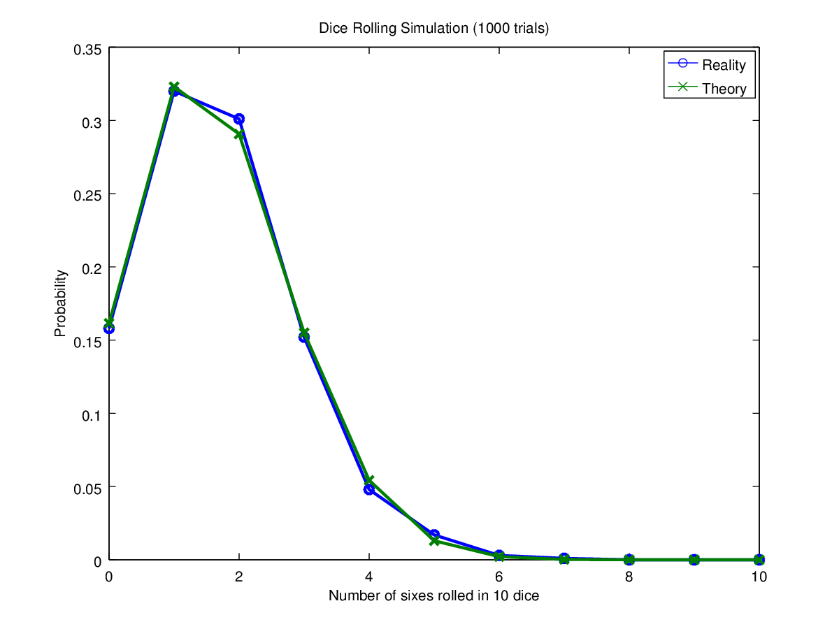
If one repeatedly threw 10 dice, in what proportion of throws would there be 0, 1, 2 ... 10 sixes. A quick burst of GNU Octave gave me an interesting if rather predictable insight in to the problem (the green line represents the theoretical result, the blue line the actual one).

After 10 trials: roughly the same shape

After 100 trials: definitely improving

After 1,000 trials: a pretty close fit

After 10,000 trials: slightly better

After 100,000 trials: the curves are practically indistinguishable

As you can see, even after 10 trials the shape is roughly right, after 100 it's beginning to more or less resemble theory and once you've done 10,000 or more it's obvious that the two match. Now the Octave code I used to generate the random dice throws is as follows (disclaimer as you can probably tell I am no expert in Octave):

 faces = 6  
 dice = 10  
 trials = 100000  
 rolls = histc(sum(randi(faces, dice, trials) == 6), 0:dice)/trials;  
 theory = binopdf(0:dice, dice, 1/faces);  

On the face of it, this is a horrendously inefficient way to do things, particularly as the value of trials increases because we allocate a trials x 10 matrix of random numbers and then go through it row by row counting the number of sixes in each and incrementing the appropriate histogram bin. Yet my workstation (a fairly ordinary Intel i5 2320 CPU @ 3.0 GHz with 8 GB of memory running Ubuntu 64-bit 14.04.2) will process 1,000,000 rows in 0.2 sec! To do this it needs to generate 10,000,000 random numbers modulo 6, count the number of sixes in 1,000,000 rows and increment a histogram bin for each row. That's pretty darned impressive and gives an insight in to how efficient Octave is under the surface.

So what happens if we unpick what Octave is doing under the surface and simply have a loop which creates a vector of random numbers 1,000,000 times.

 rolls = zeros(1, dice+1);  
 for i = 1:trials  
   rolls(sum(randi(faces, dice, 1) == 6)+1)++;  
 endfor  

Well, the short answer is it takes 135 seconds to execute. So about 600 times less efficient by going through the interpreter than letting the underlying library routines in Octave rip.

Where the Python romps...

So what of the wonderful Python and its utterly sublime companion Numpy? Well in short the following:

 import numpy  
 import numpy.random  
 import time  
 dice = 10  
 faces =  6  
 runs = 1000000  
 start = time.time()  
 k=(numpy.random.randint(faces, size=(runs, dice)) == 0).sum(axis=1)  
 b=numpy.histogram(k, numpy.arange(dice+1))  
 end = time.time()  
 print("{} rows in {:.1f} sec".format(runs, end-start))  

also took 0.2 sec to process 1,000,000 records.

So once again I tried replacing the 1,000,000 x 10 matrix with a single vector of randints:

 import numpy  
 import numpy.random  
 import time  
 dice = 10  
 faces =  6  
 runs = 1000000  
 start = time.time()  
 counters=numpy.zeros(dice+1, dtype=numpy.int32)  
 for i in range(runs):  
   k=(numpy.random.randint(faces, size=dice) == 0).sum()  
   counters[k] += 1  
 end = time.time()  
 print("{} rows in {:.1f} sec".format(runs, end-start))  

This ran in (a still quite impressive) 20.1 sec and when I abandoned Numpy and vectors altogether and used pure Python

 import random  
 import time  
 dice = 10  
 faces =  6  
 runs = 1000000  
 start = time.time()  
 counters = (dice+1)*[0]  
 for i in range(runs):  
   count = 0  
   for j in range(dice):  
     if random.randint(1, 6) == 6:  
       count += 1  
   counters[count] += 1  
 end = time.time()  
 print("{} rows in {:.1f} sec".format(runs, end-start))  

it ran in 17.9 sec, so about 90 times slower than Numpy.

Old school C

So how about some highly optimised C. That would surely perform much better than Numpy/Octave do under the surface. The answer is yes it does perform better, but not that much better.

The following took 0.11 sec to execute.

 #include <stdio.h>  
 #include <stdlib.h>  
 #include <math.h>  
 #include <time.h>  
 #include <string.h>  
 #define FACES   6  
 #define DICE   10  
 #define RUNS 1000000  
 extern int main() {  
  int i, j, counter;  
  struct timeval start, end;  
  int bins[DICE+1];  
  float t;  
  memset(bins, 0, sizeof(bins));  
  gettimeofday(&start, NULL);  
  for (i = 0 ; i < RUNS ; i++) {  
   counter = 0;  
   for (j = 0 ; j < DICE ; j++) {  
    if (rand()%FACES == 0) counter++;  
   }  
   bins[counter]++;  
  }  
  gettimeofday(&end, NULL);  
  for (i = 0 ; i <= DICE ; i++) {  
   printf("%2d %7d\n", i, bins[i]);  
  }  
  t = (float)end.tv_sec - (float)start.tv_sec + (end.tv_usec - start.tv_usec)/1000000.0;  
  printf("%d rows in %.2f sec\n", RUNS, t);  
  return 0;  
 }  

What about the memory footprint?

Well, 20-30 years ago that would have been a serious consideration, but assuming for each row we are generating 10 integers for the dice rolls and another one for the counter. Then for 1,000,000 rows we are generating 11,000,000 integers which, assuming Octave stores them as contiguous 32-bit quantities will only take up 44 MB of memory.

But... if the number of runs is too high (e.g. 1,000,000,000) then things get quite alarming. Octave just bottles and refuses to do anything. Python gamely has a go, but it soon becomes clear as the disk begins thrashing wildly that we've blown the top off the Virtual Memory.

Conclusions

1. Firstly I tip my hat to the folks behind both Numpy and Octave. Both are blindingly fast when left to their own devices, even when compared with highly-optimised custom-written C.
   
2. The speed of stuff like Numpy explains why Python is emerging as the language of choice for data-wrangling in places like LANL and has displaced things like FORTRAN.
   
3. As expected, the Python and Octave interpreters are relatively slow but in this exercise the Python interpreter was cranking out 50,000 rows per second which is quite healthy. As a side-note, the Python GIL means that multi-core programming remains difficult and I believe that this restriction also carries over to SciPy/NumPy
4. Memory footprint shouldn't be much of an issue these days, unless you are manipulating absolutely vast matrices or other structures. If it is an issue, given the compelling difference in performance between the Numnpy/Octave library routines and trying to roll your own versions in the interpreter it is still worth trying to take advantage of this performance by (if possible) breaking your data-set up in to large but manageable chunks

Bricking your super-hub with confidence!

UPDATE

I've now had the Virgin Media cable internet service for over a year and it's superb. I upgraded to the 150 Mbps service a few months back and now regularly get in excess of 160 Mbps downstream and 10 Mbps upstream. The service seems quite reliable: in a year there have been two or three dropouts and most problems are solved by resetting the cable modem.

The only problem is if you do need assistance on anything technical particularly anything Linux, DNS etc. related then be prepared to do battle with a numpty with a script in some distant Indian call centre.

13 November 2014

Introduction

I've been wanting high-speed broadband for some time and sadly my old ISP (the wonderful and extremely geek-friendly Zen Internet) are unable to provide it to my location in central Manchester any time soon. So I recently took the slightly reluctant decision to move over to Virgin Media's cable internet. The installation went ahead two days ago.

Now I have a slightly geeky setup which involves an IP PBX which I will write about in detail some other time but which has two "lines" connected to it: an ordinary analogue (POTS) phone line and a VoIP (SIP) service resold by a company called ip chitchat. This works absolutely fine and the POTS line receives inbound calls and outbound ones go out via the VoIP service. In order to get the VoIP service working originally on my old ADSL setup I had to configure my router (a Netgear DGN-1000). This was to allow incoming SIP requests to my IP PBX (NATed behind the firewall) and subsequent RTP traffic to the SIP end-point making or receiving the call. For security I restricted the source IP addresses allowed to connect to those ports to those of the VoIP servers. If you don't do this you can get a combination of either not being able to receive inbound calls or being able to make or receive a call but not getting voice in one or both directions.

The Super Hub

As part of their bundle Virgin supply a Super Hub. This is a badged/mask programmed router, firewall and wireless base-station. It's very sleek and nice looking and I'm sure it's adequate for the needs of 99% of Virgin's customers. But I'm not part of the 99%. Sadly it doesn't support VoIP nor can it be configured to as even the advanced options available in its configuration pages aren't.

The bad news is that the Super Hub acts as the cable modem: i.e. it is necessary to have it in order to connect to the cable network. So unlike ADSL you can't just bin it and get something else. However, not all is lost, but sadly this next bit will cost you money. The Super Hub comes with the option of enabling modem mode. In this mode its routing, firewall and wireless functions are disabled.

So the solution I used for my non-standard requirements was to turn the Super Hub in to a cable modem and then supply my own router, firewall and wireless base-station.

Bricking your Super Hub

Get a router

In order to get VoIP running you will need a new router. Experience of running VoIP through NetGear routers with an ADSL connection suggests that a NetGear router would do the job although I haven't tried this. I've also had a recommendation of Zyxel routers from someone else who has solved this problem on cable. I went to see my chums at MicroDirect who had a special offer on the Asus RT-N66U. This is a slightly pricey unit, but very nice.

If anyone has any recommendations or caveats about what works then I will happily maintain a list.
One thing I would advise if you are looking for a router which will handle VoIP is to make sure that when reading round the subject on-line you ignore anything which is more than a couple of years old because it is very likely out of date.

In extremis if you have a spare Gigabit Ethernet card and a Linux box or spare PC which can be turned in to one you can make your own router/firewall. This actually is considerably simpler than it sounds, but of course still gives you the problem of not being a wireless base-station.

Now brick your Super Hub

If you've spent any time configuring the Super Hub already (e.g. with a different address range, DHCP pool etc.) then it it probably worth backing up the configuration before you do anything else. 
So, to brick your Super Hub (and please note that this is for information only, this worked fine for me, but don't blame me if it doesn't for you etc.) follow the instructions on the Virgin website.
This will turn your Super Hub in to a cable modem, turning off the routing and wireless features. So note that as soon as you do this you will lose internet access so if you are likely to need to look anything up make sure you've loaded it in advance.


Also note that when the Super Hub is bricked in to modem mode its DHCP server no longer works and its IP address changes to 192.168.100.1.

Configure your router

You will need to connect the WAN port of your router to the MODEM port on the Super Hub (the other ports are disabled). All I needed to do on the Asus router was set the WAN connection type to Automatic IP (as opposed to PPoE etc.) and it sprung in to life.

Alternatively if this doesn't work you  may also need to set the WAN IP address on your router manually to something in the range 192.168.100.0/24 with subnet mask 255.255.255.0 and default gateway 192.168.100.1 and primary and secondary DNS of 194.168.4.100 and 194.168.8.100.

I also configured the DHCP server to allocate exactly the same addresses to the various devices on my LAN as under the previous regime.

So we now have:

Configure your firewall

Having paid for the router I was disappointed to read various (old) postings about trouble getting Asus routers working with VoIP and I was dismayed that I couldn't find anything obvious in the Asus's web-based configuration which allowed me to permit various inbound IP addresses through the firewall. But to my amazement it just worked. First time. Without any special configuration. I could make and receive VoIP calls with bidirectional voice. Evidently the Asus firmware must have been updated since the earlier posts and now it just "understands" VoIP.

Your mileage may vary, particularly depending upon the manufacturer and model of router you are using. But I'm a very happy customer.

Test your configuration

As with any activity which potentially opens up the firewall on an internet-connected router you should always check security (particularly if it works suspiciously easily out of the box as above).
That would be another article some other time but a good place to start is to do a port-scan using the excellent Shields Up application from GRC.

The result

When I was using the Super Hub as combined router, firewall and modem I was getting about 80 Mbps downstream out of it. Obviously these figures vary considerably, but with the Asus unit I'm consistently getting about 100 Mbps. Whether this is due to better performance by the LAN or WAN side of the router I have no idea.

If it all goes horribly wrong

Other than the expense of getting a router (use a reliable supplier who will give you your money back or a credit note), you can always restore the Super Hub to its former state by turning off modem mode or if it's dead by using a paperclip to press and hold the reset button for about 20 sec until the lights flash on the Ethernet ports.