I use
GNU Octave as a sort of very powerful desktop calculator, and a couple of days ago I was musing about the
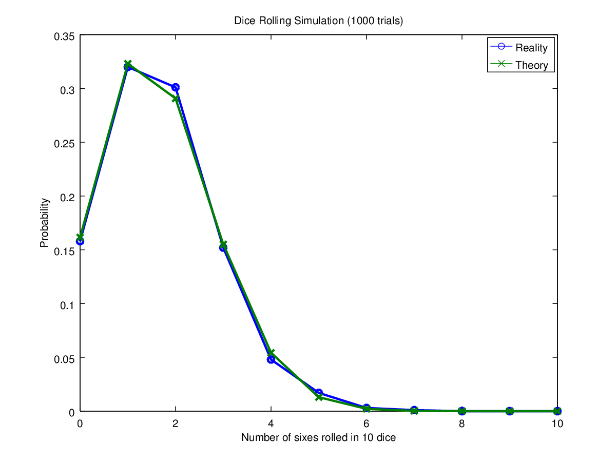
binomial probability distribution and how many trials one would have to perform before the observed results began to mirror the theory. This led me to consider the following experiment.
If one repeatedly threw 10 dice, in what proportion of throws would there be 0, 1, 2 ... 10 sixes. A quick burst of GNU Octave gave me an interesting if rather predictable insight in to the problem (the green line represents the theoretical result, the blue line the actual one).
 |
| After 10 trials: roughly the same shape |
 |
| After 100 trials: definitely improving |
 |
| After 1,000 trials: a pretty close fit |
 |
| After 10,000 trials: slightly better |
 |
| After 100,000 trials: the curves are practically indistinguishable |
As you can see, even after 10 trials the shape is roughly right, after 100 it's beginning to more or less resemble theory and once you've done 10,000 or more it's obvious that the two match. Now the Octave code I used to generate the random dice throws is as follows (disclaimer as you can probably tell I am no expert in Octave):
 faces = 6
 dice = 10
 trials = 100000
 rolls = histc(sum(randi(faces, dice, trials) == 6), 0:dice)/trials;
 theory = binopdf(0:dice, dice, 1/faces);
On the face of it, this is a horrendously inefficient way to do things, particularly as the value of
trials increases because we allocate a
trials x 10 matrix of random numbers and then go through it row by row counting the number of sixes in each and incrementing the appropriate histogram bin. Yet my workstation (a fairly ordinary Intel i5 2320 CPU @ 3.0 GHz with 8 GB of memory running Ubuntu 64-bit 14.04.2) will process
1,000,000 rows in
0.2 sec! To do this it needs to generate 10,000,000 random numbers modulo 6, count the number of sixes in 1,000,000 rows and increment a histogram bin for each row. That's pretty darned impressive and gives an insight in to how efficient Octave is under the surface.
So what happens if we unpick what Octave is doing under the surface and simply have a loop which creates a vector of random numbers 1,000,000 times.
 rolls = zeros(1, dice+1);
 for i = 1:trials
   rolls(sum(randi(faces, dice, 1) == 6)+1)++;
 endfor
Well, the short answer is it takes 135 seconds to execute. So about 600 times less efficient by going through the interpreter than letting the underlying library routines in Octave rip.
Where the Python romps...
So what of the wonderful
Python and its utterly sublime companion
Numpy? Well in short the following:
 import numpy
 import numpy.random
 import time
 dice = 10
 faces =  6
 runs = 1000000
 start = time.time()
 k=(numpy.random.randint(faces, size=(runs, dice)) == 0).sum(axis=1)
 b=numpy.histogram(k, numpy.arange(dice+1))
 end = time.time()
 print("{} rows in {:.1f} sec".format(runs, end-start))
also took 0.2 sec to process 1,000,000 records.
So once again I tried replacing the 1,000,000 x 10 matrix with a single vector of randints:
 import numpy
 import numpy.random
 import time
 dice = 10
 faces =  6
 runs = 1000000
 start = time.time()
 counters=numpy.zeros(dice+1, dtype=numpy.int32)
 for i in range(runs):
   k=(numpy.random.randint(faces, size=dice) == 0).sum()
   counters[k] += 1
 end = time.time()
 print("{} rows in {:.1f} sec".format(runs, end-start))
This ran in (a still quite impressive) 20.1 sec and when I abandoned Numpy and vectors altogether and used pure Python
 import random
 import time
 dice = 10
 faces =  6
 runs = 1000000
 start = time.time()
 counters = (dice+1)*[0]
 for i in range(runs):
   count = 0
   for j in range(dice):
     if random.randint(1, 6) == 6:
       count += 1
   counters[count] += 1
 end = time.time()
 print("{} rows in {:.1f} sec".format(runs, end-start))
it ran in 17.9 sec, so about 90 times slower than Numpy.
Old school C
So how about some highly optimised C. That would
surely perform much better than Numpy/Octave do under the surface. The answer is yes it does perform better, but not that much better.
The following took 0.11 sec to execute.
 #include <stdio.h>
 #include <stdlib.h>
 #include <math.h>
 #include <time.h>
 #include <string.h>
 #define FACES   6
 #define DICE   10
 #define RUNS 1000000
 extern int main() {
  int i, j, counter;
  struct timeval start, end;
  int bins[DICE+1];
  float t;
  memset(bins, 0, sizeof(bins));
  gettimeofday(&start, NULL);
  for (i = 0 ; i < RUNS ; i++) {
   counter = 0;
   for (j = 0 ; j < DICE ; j++) {
    if (rand()%FACES == 0) counter++;
   }
   bins[counter]++;
  }
  gettimeofday(&end, NULL);
  for (i = 0 ; i <= DICE ; i++) {
   printf("%2d %7d\n", i, bins[i]);
  }
  t = (float)end.tv_sec - (float)start.tv_sec + (end.tv_usec - start.tv_usec)/1000000.0;
  printf("%d rows in %.2f sec\n", RUNS, t);
  return 0;
 }
What about the memory footprint?
Well, 20-30 years ago that would have been a serious consideration, but assuming for each row we are generating 10 integers for the dice rolls and another one for the counter. Then for 1,000,000 rows we are generating 11,000,000 integers which, assuming Octave stores them as contiguous 32-bit quantities will only take up 44 MB of memory.
But... if the number of runs is too high (e.g. 1,000,000,000) then things get quite alarming. Octave just bottles and refuses to do anything. Python gamely has a go, but it soon becomes clear as the disk begins thrashing wildly that we've blown the top off the Virtual Memory.
Conclusions
- Firstly I tip my hat to the folks behind both Numpy and Octave. Both are blindingly fast when left to their own devices, even when compared with highly-optimised custom-written C.
- The speed of stuff like Numpy explains why Python is emerging as the language of choice for data-wrangling in places like LANL and has displaced things like FORTRAN.
- As expected, the Python and Octave interpreters are relatively slow but in this exercise the Python interpreter was cranking out 50,000 rows per second which is quite healthy. As a side-note, the Python GIL means that multi-core programming remains difficult and I believe that this restriction also carries over to SciPy/NumPy
- Memory footprint shouldn't be much of an issue these days, unless you are manipulating absolutely vast matrices or other structures. If it is an issue, given the compelling difference in performance between the Numnpy/Octave library routines and trying to roll your own versions in the interpreter it is still worth trying to take advantage of this performance by (if possible) breaking your data-set up in to large but manageable chunks